Getting started with OpenCV in Python

Armando Anaya

Published on June 22, 2024

If you have no experience working with OpenCV in Python and want to learn how to use its basic functions to explore this powerful computer vision tool, this article is for you. I'll explain the main functions of OpenCV, the essential concepts about images you need to know, and how this library handles images as NumPy arrays.

To get started, you must install the OpenCV library in your Python environment. If you prefer to conduct these tests in Google Colab, installing the library is unnecessary, as it is preinstalled in that environment.

1pip install opencv-python

Once installed, you can import the library into your project as follows:

1import cv2
2print(cv2.__version__)

If the OpenCV version is successfully displayed, this indicates that you have OpenCV installed and ready to use.

Additionally, to facilitate learning, we have prepared a Jupyter Notebook that is available in our public GitHub repository. This notebook is designed to guide you efficiently through the practices described in this article. You can access the Notebook and copy it to your Google Colab account using the following link (Jupyter Notebook).

Opening the First Image

Opening images with OpenCV and converting them into manipulable objects for our programs is a relatively straightforward process. Before using the specific OpenCV function for this, it's crucial to understand how this operation is carried out.

First, it's important to comprehend how OpenCV handles images in Python. If you are not familiar with NumPy, an essential library for managing arrays and tensors, here's a brief explanation: NumPy facilitates working with matrix data structures, allowing for complex operations such as mathematical calculations, linear algebra algorithms, matrix shape manipulation, and submatrix extraction. NumPy is significantly more efficient in these operations than Python's native data structures, such as nested lists.

Understanding NumPy is essential, as OpenCV consistently uses this library. When loading an image, OpenCV does not return an instance of some proprietary object but rather a three-dimensional NumPy array representing the image's width, height, and color channels. This data manipulation method is very advantageous in Python, mainly for compatibility with machine learning frameworks like Scikit-Learn, Keras, or PyTorch.

When opening an image, you can load it in one of three possible color spaces:

1cv2.IMREAD_COLOR
2cv2.IMREAD_GRAYSCALE
3cv2.IMREAD_UNCHANGED

OpenCV uses one of these modes as the second parameter in its loading function. By default, cv2.IMREAD_COLOR loads the image in RGB color space (although OpenCV handles this format as BGR, which will be detailed later). The grayscale option loads the image with a single color channel, while cv2.IMREAD_UNCHANGED allows image loading with all color channels defined in the original format, including the alpha channel, for transparency in images like PNG.

The process of loading a color image in JPG format is simple. First, we download the image we will be working with:

1wget -q --show-progress https://img.freepik.com/free-photo/selective-focus-shot-adorable-german-shepherd_181624-30217.jpg -O dog.jpg

Then, we load it with the corresponding function:

1image = cv2.imread("dog.jpg", cv2.IMREAD_COLOR)

With this, we have created an image object containing the corresponding NumPy array.

If you are following the instructions in our Notebook, there we explain how to display the image in OpenCV. If you want to show the image from a program on your computer, you can use the following function, which will open a window with the image until you press any key to close it:

1# Display the image in the window until any key is pressed
2cv2.imshow("Dog", image)
3cv2.waitKey(0)
4cv2.destroyAllWindows()

The RGB Color Space in OpenCV

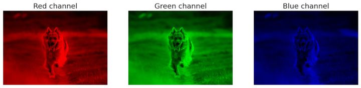
When working with images in OpenCV, it is essential to familiarize yourself with the concept of color spaces. This is a broad topic, but for now, it's enough to understand that when we mention RGB, we refer to the color space that divides the image into three channels: red (R), green (G), and blue (B). Each channel corresponds to the pixel data for each color, and by combining these three channels, we get the colorful images we are accustomed to. By default, OpenCV loads color images as BGR, not RGB, meaning the red and blue channels are reversed. This can confuse, as some third-party libraries expect the channels in RGB order, while native OpenCV functions, like imshow for displaying images, expect BGR.

This peculiarity of OpenCV is due to historical reasons. When the library was initially developed, there was no clear standard on the order of the channels in the array, and some digital camera companies stored their images in BGR space by default. The developers of OpenCV chose this format to work with images, and it has been maintained for reasons of backward compatibility.

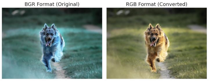
To convert the color space of an image from BGR to RGB, we use the cvtColor function. The two parameters of this function are the image object and a flag that indicates the type of transformation to perform. There are many possible color space transformations, but for now, we will focus on switching from BGR to RGB:

1image_rgb = cv2.cvtColor(image, cv2.COLOR_BGR2RGB)

This image_rgb object will be the reference in the following examples and is also available in our exercise Notebook for consultation.

Manipulating the Image

OpenCV is one of the most powerful computer vision libraries available today, offering a wide range of functions and options for manipulating images. Next, we will highlight some of the fundamental operations that every user should know.

The essential functions we will explore include:

• Resizing the image
• Rotating the image
• Flipping the image
• Cropping the image
• Changing the image's color space
• Adding text to the image
• Drawing shapes on the image

We will proceed to describe each of these functions in detail:

Resizing the Image

Resizing an image in OpenCV is a straightforward process thanks to the resize function, which operates with two main parameters. The first is the image object, and the second is a tuple that specifies the new desired dimensions. For example:

1image_resized = cv2.resize(image, (240, 240))

Additionally, the resize function allows proportional adjustments to the current size of the image, making it easy to increase or decrease the size by a specific percentage. For example, to reduce the size of an image by 50%, you can use the following configuration:

1small_image = cv2.resize(image_rgb, (0,0), fx=0.5, fy=0.5)

Similarly, to double the size:

1big_image = cv2.resize(small_image, (0,0), fx=2, fy=2)

It's important to note that when using the fx and fy parameters for proportional scaling, the size tuple is declared with zeros to meet the function's requirements, making specific dimensions irrelevant.

Rotating the Image

Rotating an image in OpenCV is a fundamental operation similar to resizing. The rotate function of OpenCV is quite intuitive and requires only two parameters: the image object and the flag that specifies the rotation type. This function allows rotations in multiples of 90 degrees, including 90 degrees to the right, left, or 180 degrees.

Rotate 90 degrees to the right:

1rotated_image = cv2.rotate(image_rgb, cv2.ROTATE_90_CLOCKWISE)

Rotate 90 degrees to the left:

1rotated_image_2 = cv2.rotate(image_rgb, cv2.ROTATE_90_COUNTERCLOCKWISE)

Rotate 180 degrees:

1rotated_image_3 = cv2.rotate(image_rgb, cv2.ROTATE_180)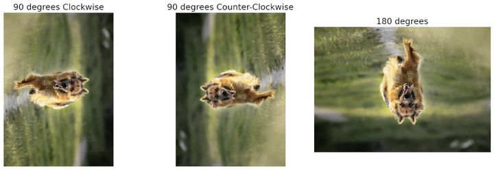

For angles that are not multiples of 90 degrees, such as 45 degrees, we use getRotationMatrix2D and warpAffine:

1rotation_matrix = cv2.getRotationMatrix2D((image_rgb.shape[1] / 2, image_rgb.shape[0] / 2), 45, 1)
2rotated_image_4 = cv2.warpAffine(image_rgb, rotation_matrix, (image_rgb.shape[1], image_rgb.shape[0]))

Flipping the Image

Flipping an image is another fundamental operation in OpenCV, especially useful in preprocessing images for training neural network models. This operation is performed with the flip function, which accepts a parameter to indicate the axis:

To flip horizontally:

1image_flipped_horizontal = cv2.flip(image_rgb, 1)

To flip vertically:

1image_flipped_vertical = cv2.flip(image_rgb, 0)

Cropping the Image

Cropping an image is a fundamental technique in image processing that allows focusing on or removing specific areas of an image. In OpenCV, cropping is handled somewhat differently, as there is no specific function dedicated to this task. Instead, we utilize the matrix manipulation capabilities of NumPy, taking advantage of OpenCV and treating images as NumPy arrays.

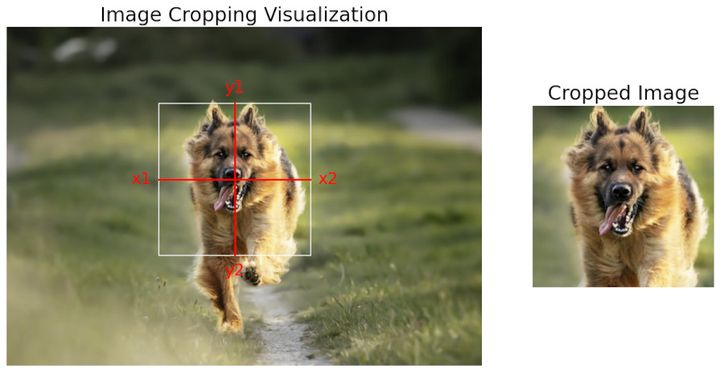
To crop an image, we specify the coordinates of the cropping rectangle directly in the matrix indices. The indices on the x-axis (horizontal) and y-axis (vertical) determine the section of the image we wish to extract:

1cropped_image = image_rgb[100:300, 200:400]

In this example, 100:300 represents the range on the y-axis, selecting from pixel 100 to pixel 299, and 200:400 represents the range on the x-axis, selecting from pixel 200 to pixel 399. This results in a crop that forms a vertical rectangle starting at the point (200, 100) and extending to the point (399, 299).

This cropping method is highly efficient in terms of performance due to how NumPy handles operations on arrays. It allows great flexibility in selecting specific areas of an image without additional complicated functions. Moreover, knowing how to manipulate arrays with NumPy opens the door to various other image-processing operations, making it a valuable skill in computer vision.

Changing the Color Space

In another publication, we will delve deeper into the topic of color spaces, as understanding them is crucial in computer vision. For now, we will exemplify one of the most commonly used transformations in practice with OpenCV: converting a color image to a grayscale. Similar to converting an image from BGR to RGB, we will use the cvtColor() function. However, this time, we will use the flag that allows converting an RGB image to grayscale:

1gray_image = cv2.cvtColor(image_rgb, cv2.COLOR_RGB2GRAY)

Adding Text to the Image

Adding text to images with OpenCV is a commonly used technique in object labeling, especially in projects involving machine learning models for object detection. Next, we will explore how to use the cv2.putText() function to incorporate text into an image. It is crucial to remember that this function directly modifies the image passed as a parameter, so if you want to keep the original image unchanged, it is necessary to copy it before applying the text. The parameters required by this function include:

• Image object.
• Text to insert.
• Tuple with coordinates where the text is to be inserted.
• Font type.
• Font scale, which is a factor in adjusting the text size.
• Text color.
• Text line thickness.
• Line type.

The following code illustrates how to insert text into an image using all the mentioned parameters:

1# Copy the original image because we will draw on it, and it
2# will modify the original image
3image_with_text = image_rgb.copy()
4
5# Select the font to use
6font = cv2.FONT_HERSHEY_SIMPLEX
7
8cv2.putText(image_with_text, "Hello, I'm a dog! Woof!", (10, 50), font, 1, (255, 255, 255), 2, cv2.LINE_AA)

The result can be visualized immediately afterward in the processed image.

Drawing Shapes on the Image

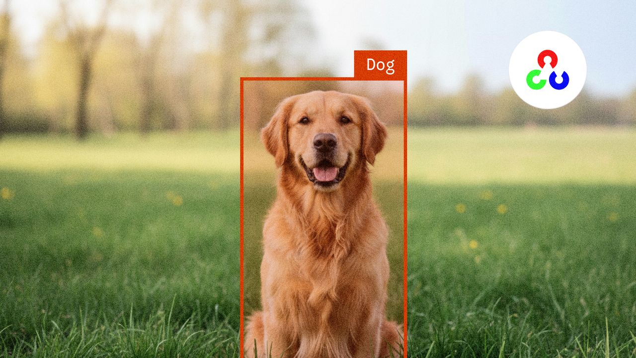
Adding geometric shapes to images is a common practice in image processing with OpenCV, especially useful in computer vision applications like object detection. A frequent use of this capability is to draw bounding boxes around objects identified by deep learning algorithms, such as YOLO (You Only Look Once), to visualize the location and scope of the detection.

For example, to draw a rectangle around a detected object in an image, such as a dog, we use the cv2.rectangle() function. Below is how you might draw a rectangle that delineates the dog from the point (218, 90) to the point (404, 412):

1image_with_rectangle = image_rgb.copy()
2
3cv2.rectangle(image_with_rectangle, (218, 90), (404, 412), (255, 0, 0), 2)

This rectangle is drawn in red with a thickness of 2 pixels. Additionally, adding text labels to the bounding boxes to identify the detected object is common, simulating a typical prediction from an object detection algorithm. Here's how to add the label "Dog" to the bounding box we just drew:

1image_with_rectangle = image_rgb.copy()
2color_red = (255, 0, 0)
3
4cv2.rectangle(image_with_rectangle, (218, 90), (404, 412), color_red, 2)
5
6font_size = 0.7
7font = cv2.FONT_HERSHEY_SIMPLEX
8
9cv2.putText(image_with_rectangle, "Dog", (218, 80), font, font_size, color_red, 2, cv2.LINE_AA)

The label "Dog" is placed just above the rectangle, using the same red color to maintain visual consistency. These operations help improve the visual interpretation of the algorithm's results and are essential for tuning and evaluating object detection models in development and production environments.

These OpenCV tools enable effective integration of visualization into machine learning processes, enhancing human interaction with model results and facilitating the understanding and analysis of processed data.